

Snowflake is widely praised for its scalability and performance, but cost control often remains a black box. Many teams rely on simplified query cost estimates that don’t reflect how Snowflake actually bills usage. In this post, we’ll break down the underlying factors that drive cost per query and show how a more accurate method can lead to smarter optimization and lower spend.
Decoding Snowflake cost per query
Several key components contribute to your Snowflake bill: compute usage, query complexity, execution plans, and supporting services. For most users, compute costs represent the largest portion of total spend. Understanding how these costs are incurred is crucial for effective optimization.
Compute costs: virtual warehouse size and runtime
Virtual Warehouses are Snowflake’s core compute engines, built as massively parallel processing clusters. Each cluster consists of multiple virtual machines and offers elastic, horizontal scaling. Snowflake doubles processing power, memory, and SSD capacity with each increase in warehouse size, ensuring predictable and linear performance scaling.
While larger warehouses do incur higher costs per unit of time, a common misconception is that bigger always means more expensive. In reality, larger warehouses can often reduce total cost of ownership by completing queries faster and more efficiently. It’s essential to evaluate the full picture: query complexity, execution plan, and overall load all influence true cost.
Warehouse and cluster size determine the resources available per query. Importantly, Snowflake charges based on warehouse uptime, not query duration. This means query concurrency significantly impacts cost calculations.
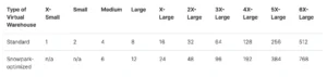
See credit map illustrating warehouse sizes, available resources per query, and corresponding credit costs.
Larger warehouses offer more memory and processing power, allowing for faster execution—if the query plan can leverage parallelization. Once the limit of parallel execution is reached, additional resources provide diminishing returns and can drive up costs unnecessarily.
Compute costs: concurrency
Another key factor influencing query cost is concurrency. An X-Small (XS) warehouse is powered by one virtual machine with 8 cores. As warehouse sizes grow, the number of cores increases—but the default concurrency limit remains 8 queries, whether using XS or 6XL.
Concurrency can be adjusted via the MAX_CONCURRENCY_LEVEL parameter or by increasing cluster count. For example:
- If MAX_CONCURRENCY_LEVEL is set to 8, one active cluster handles 8 parallel queries.
- If two clusters are active, the limit doubles to 16 parallel queries.
However, it’s uncommon and risky,to increase MAX_CONCURRENCY_LEVEL beyond 8. While technically possible, doing so often results in performance degradation due to queuing. We’ve observed multiple use cases where increasing it to 24 or 32 caused noticeable slowdowns.
Calculating cost per query
Flawed approach
The most common (and incorrect) way to calculate cost per query is to look at query duration in isolation and multiply it by the warehouse’s per-hour cost. For example:
- 1-minute query on an X-Small warehouse (1 credit/hour) = 1/60 x $3 = $0.05
This is flawed for two reasons:
- Concurrency Ignored: Multiple queries may be running at once. Since Snowflake bills uptime, not per-query runtime, the cost is overestimated.
- Auto-Suspend Ignored:A single 1-second query may trigger several minutes of billed time if auto-suspend is set to 300 seconds, underestimating the cost.
In short, this method produces skewed results.
Improved method
Since billing is based on warehouse uptime, a more accurate approach allocates costs based on that uptime. Here’s how we do it at Seemore Data:
- Treat each warehouse uptime as a single event.
- Group all queries that ran during that uptime.
- Calculate total query duration.
- Allocate a percentage of total time to each query.
- Multiply those percentages by total warehouse uptime to get “normalized query runtimes.”
- Apply cost per second based on warehouse type and compute the “normalized cost per query.”
This method correctly accounts for concurrency, idle time, and avoids the distortion seen in simpler models.
Let’s walk through a real example:
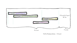
- A Small warehouse runs for 53 seconds.
- Query processing takes 38 seconds, with 10 seconds of idle time.
Queries:
- Query 1: 10s
- Query 2: 24s
- Query 3: 4s
- Query 4: 6s
- Total query duration: 44s
Percentage allocation:
- Q1: 22%
- Q2: 55%
- Q3: 9%
- Q4: 14%
Normalized query runtimes:
- Q1: 12s
- Q2: 29s
- Q3: 5s
- Q4: 7s
Cost per second (Small warehouse @ 2 credits/hour = $6/hour = $0.0017/second):
- Q1: 12s x $0.0017 = $0.02
- Q2: 29s x $0.0017 = $0.05
- Q3: 5s x $0.0017 = $0.008
- Q4: 7s x $0.0017 = $0.012
Check:
- Total warehouse cost: 53s x $0.0017 = $0.09
- Sum of query costs: $0.02 + $0.05 + $0.008 + $0.012 = $0.09
✅ Aligned.
Why this matters
Snowflake’s pricing model rewards efficient resource usage,but only if you understand how it works. Simple cost-per-query estimates often lead teams astray, inflating or underestimating expenses and obscuring optimization opportunities. By using a normalized, warehouse-uptime-based approach, you get a clearer picture of true query costs,and a better foundation for cost control.
What to do next
If you’re aiming to lower your Snowflake spend without compromising performance, precision matters. At Seemore Data, we specialize in uncovering the real story behind your warehouse metrics. Want to see how much you could save? Schedule a consultation with our data optimization experts today.